In part 1 of this post, we have seen how a simple parameter sweep can be used to explore the relationship between decision variables and KPIs as well as between conflicting objectives, like maximizing service level and maximizing profit.
Here we show how it can be used to decide between a maximal but uncertain profit and a less ambitious but also more predictable one.

Maximal or most robust profit?

In a previous post, we briefly showed how Cosmo Tech CoMETS can be used on a supply chain digital twin to automatically optimize profit in an uncertain demand context.

However, in many situations, we are not only interested in the best strategy on average but also in the one whose performance is the least uncertain. Therefore, we may want to look for a more robust strategy, that is less variable, even if it may not provide the maximal expected benefit.

Variability of a key performance indicator (KPI) can be measured by its “dispersion” or “standard deviation” in an uncertainty analysis. Since CoMETS allows you to combine experiments, you could embed an uncertainty analysis within an optimization asking to minimize the dispersion (instead of maximizing the mean profit). However, the trivial solution here would just be to keep the inventory always empty and never serve any demand: the profit will never vary but be always minimal (which is what CoMETS would prescribe if you do this).

Multi-objective optimization problem

Actually, you don’t want a strategy that either maximizes profit or minimizes risk. You want something able to handle both simultaneously (like for profit and service level objectives). This may not be possible actually because these are often contradictory objectives.

Here, you also have a multiobjective optimization problem. In a future CoMETS version, we will introduce automatic multiobjective optimization, but for now we will use a simpler approach. One of the simplest techniques is to define a single objective made up of a weighted sum of the multiple objectives.

For instance, since the dispersion (or standard deviation) is a measure of the variability, we could decide to maximize the mean expected profit discounted by its dispersion (we give the same weight to the profit maximization and to the variability minimization): in this way, an increased dispersion adds a penalty to the profit maximization¹. So as before, we create a “robust” objective with an uncertainty analysis experiment to be embedded within an optimization one, which creates a robust (or stochastic) optimization:

Objective set to “mean profit – profit standard deviation”.

As expected, the result is a reduced dispersion (or uncertainty): 995 instead of 1494 for the previous optimization, but a the cost of a reduced profit (4938 vs. 5100):

Profit statistics from the “multi-objective optimization”.

The following chart summarises the results obtained for the different experiments:

Mean profit +/- standard deviation for the simple optimization (“Optim”), the stochastic optimization (“Robust Optim”) (see previous post) and the combined objective optimization (“Multi Optim”).

So far we have put the same importance to the mean profit and to the profit variability. However, depending on your sector or your company’s policy, you may be more or less risk averse and decide to put different weights to each objective.

Combine uncertainty analysis with parameter sweep to adjust profit / risk ratio

Here, as in the first part of this post, we are adjusting two decision variables only (the reorder point and the reorder quantity of Retailer 1). This means that exploring their full domain of variation is not very time consuming: a parameter sweep can be used in place of an optimization, and this provides more information at the same time.

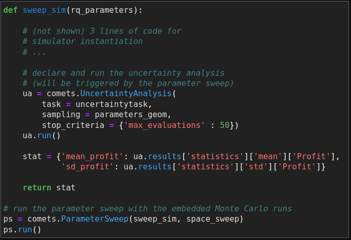
The code is very similar to the robust optimization: here we embed an uncertainty analysis within a parameter sweep.

Finally visualizing all the results on a “Profit dispersion” vs. “Mean profit” plot we can visualize the trade-off between being maximally profitable and being maximally robust to demand variations:

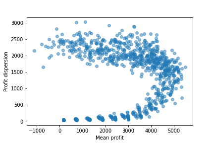
Profit dispersion vs. Mean profit. Each dot represents one of the 10000 uncertainty analyses. For each of them, the dot coordinates are the obtained mean profit and profit standard deviation. 

Very often, the variability of an indicator tends to increase with its mean value. Here we can observe that this is not the case: the relationship between the expected profit and its dispersion is not linear, nor is it monotonous. Simple linear models, like the ones generally used in supply chain modeling, would not be able to capture this pattern correctly, which is why dynamic simulation is necessary.

Since you have simulated all the possible policies, you can now select one which, though it would generate some smaller profit than the previous one, would advantageously be much less uncertain.

Here, for instance, putting the reorder point to 66 and the reorder quantity to 27 would be a much more robust, while also quite profitable, strategy as shown in the following chart:

Mean profit +/- standard deviation obtained with the different experiments. The variability of the strategy chosen from the parameter sweep (“Sweep Optim”) is much smaller than that of the other strategies.

Conclusion

Automated experiments like Optimization, Uncertainty Analysis and even a seemingly “simpler” Parameter Sweep, can provide very valuable insights, especially in an increasingly volatile world where resilience and robustness are becoming “the” only keys. Such advanced prescriptive analyses can now be carried out efficiently in a few lines of codes with CoMETS and deployed together with a Simulation Digital Twin within intuitive web-based applications to finally serve decision makers.

To go further, you can look at CoMETS release notes and dive into CoMETS documentation.

In future posts we will show how a Sensitivity Analysis can help identify the most critical parts of supply chains and how synthetic data and reinforcement learning can automate the creation of “resilient by design” policies.

Footnotes

¹ Note that there are many possible indicators of robustness and risk. Here, we want to minimize the variability or maximize the predictability of profit. Another risk minimization strategy could be for instance to minimize the probability of bad performance or maximize the worst (e.g. 10% lowest) performance.