Introduction

CoMETS is a low code Python library for very easily interacting and experimenting with numerical models and simulators and running advanced prescriptive analyses.

Different types of “Experiments” are already available such as: Optimization, Sensitivity analysis, Uncertainty Analysis, Reinforcement learning.

The Parameter Sweep in CoMETS is an experiment which allows exploring the influence of a set of parameters on key performance indicators (KPIs).

It is very useful when you need to better understand the behavior of your system, understand the joint effect of a few number of levers or test your intuition. It predicts how your system will respond when you move the value of some levers. It is best adapted to the analysis or the tuning of a single lever or a limited number of levers, in which case it can even be used in place of a more sophisticated optimization algorithm, as we will see in this post¹.

However, it can also be used with many levers, for instance, as a means for generating very large synthetic data for surrogate modeling or more generally to further train and test machine learning models when you lack historical or unbiased representative samples of possible futures.

In this post, we briefly show how a CoMETS Parameter Sweep experiment can be used with a supply chain digital twin to explore:

1. the impact on service level of the settings of a stock replenishment policy
2. the existing trade-offs between profit and service level
3. the existing trade-offs between maximal profit and profit variability given demand uncertainty (see Part 2 of the post).

Example of a digital twin that can be built and simulated with the Cosmo Tech platform

Impact of the reorder point and the reorder quantity on the KPIs

We consider a simple supply chain and we are interested in the performance of one retailer.

Previously, we showed how profit can be optimized by adjusting the parameters controlling the stock replenishment policy of Retailer 1’s inventory: the reorder point, defining which stock level threshold triggers a new order, and the associated reorder quantity.

Imagine now that you are also interested in improving some additional KPIs, like the level of service for instance, i.e. the proportion of satisfied orders, which you are asked to keep high enough, let’s say at least 90%. To achieve this goal, you may first wish to examine how the supply chain performance will change when the policy is modified within an allowed domain.

To do so, you can define the allowed exploration space (variation ranges for each parameter and total number of samples), then create and run a “parameter sweep” experiment:

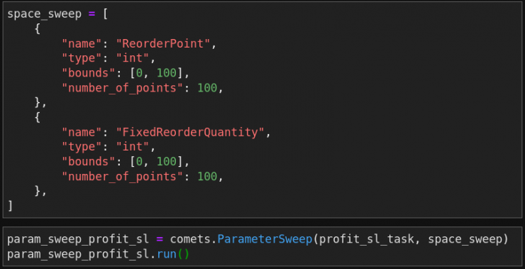
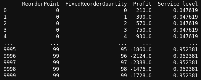
Parameter sweep with CoMETS. CoMETS will generate 100×100 = 10000 samples made up of all the combinations of ReorderPoint and FixedReorderQuantity evenly spaced between 0 and 100. (Here, profit_sl_task is the digital twin configured so that it predicts profit and service level as a function of ReorderPoint and FixedReorderQuantity)

You can then plot the results to visualize, for example, the influence of the reorder quantity on the level of service:

Effect of the order quantity on the service level for five selected reorder point values (among the 100 simulated).

Such parameter space exploration can help confirm expectations, or on the contrary, identify unintuitive behaviors, which should trigger additional analyses. Here, we can observe that, with the current supply chain settings, the service level is always 0, insensitive to the order quantity and to the reorder point when the order quantity is below a critical value. Above that value, the service level tends to rapidly raise with the order quantity.

Going further, you can also visualize how the two levers together influence both the service level and the profit:

Service level as a function of reorder point and order quantity.

Profit as a function of reorder point and order quantity.

As could be expected², we observe that you cannot simultaneously maximize the profit and the level of service since their respective maximums lie in different areas of the parameter space.

Profit – service level trade off

Finally, since for each possible combination of reorder point and reorder quantity values, you have already generated the resulting profit and service level expected values, you can directly plot the relationship between these two KPIs so as to explicitly see the trade-offs:

Profit vs. Service level (when the parameters of the replenishment policy are varied). Gray dots: results of the 10⁴ simulations (for each simulation, characterized by a unique pair of reorder point and reorder quantity, the dot represents the service level, in abscissa, and the profit, in ordinate, that are obtained for this pair); blue line: Pareto front, i.e. the relationship between the maximal profit and the maximal service level; orange dot: maximal profit for a service level not less than 90%.

The most external dots on the chart (connected through the blue line) represent the trade-off between profit and service level, or the so-called “Pareto front”: starting from any of these points, a decision increasing the level of service can only be done at the expense of a decreased profit, and vice versa.

Now, if you were asked to find a strategy that would lead to a service level larger than the minimal acceptable value of 90% (i.e. within the area located on the right-hand-side of the dashed line in the above chart), then you could also select the one that would give the highest profit compatible with this constraint, which is here 4470 (orange dot).

Conclusion

Automatic Parameter Sweep is a simple but very useful experiment to explore tendencies and trade-offs. In the second part of this post, we will see how CoMETS can be used to seamlessly combine it with an Uncertainty Analysis and explore the relationship between maximal profit and profit uncertainty.

Footnotes

¹ Actually, it is similar to the “Grid Search” approach used in machine learning to tune “hyperparameters”.
² Indeed, the higher inventory levels, necessary to serve more customers in time, also increase storage costs.