
Articles
Imagine you are a supply chain manager, your goal is to make sure the supply chain can service its customers, while keeping costs as low as possible. A central aspect of this process is to decide on the amount of inventory you should carry: if your inventory level is too low, you will not be able to meet the demand of your customers, but a too high inventory level will incur unnecessary costs.
Your task is complicated by the fact that the demand is uncertain and highly volatile. Since it takes time to react to variations in the demand of your customers, you use safety stocks to absorb surges in demand. An extremely high safety stock will ensure that all demands are served, no matter the size of a demand surge, but at a very high cost. If safety stock is too low, each time the demand is higher than expected a large number of customers will not have their demand served. To manage this tradeoff, you set a target on the service level you want to achieve, that is the proportion of the demand you want to be able to serve, for example 95 percent.
Traditionally, you have relied on safety stock formulas to decide on the right amount of safety stock to reach a particular service level. In this post we will explain what these formulas are, under which circumstances they can be applied and the limitations they have. We will then present another approach to setting safety stock levels that relies on simulation. By simulating your supply chain, you can remove the limitations that apply to safety stock formulas and make sure your safety stock is adapted to your particular supply chain. Finally we will see how optimization by simulation can automatically prescribe the right safety stock for your needs.
For concreteness we will imagine that you are a retailer selling household appliances, such as refrigerators. Each day you receive a certain amount of demand for refrigerators from your customers. You can reorder refrigerators to your supplier, and it takes a certain amount of time – the lead time – for your order to be satisfied and the refrigerators to arrive in your inventory.
If the demand were always the same, say 100 refrigerators per day, and the lead time were always of 15 days, you would not need to carry safety stock: you would reorder new refrigerators to your supplier whenever your inventory level reaches 1500. In the 15 days it takes for the new refrigerators to arrive, you would sell exactly 100×15 = 1500 refrigerators (Figure 1). Your inventory would therefore be replenished just as it reaches zero: there is no excess stock and you are always able to satisfy the demand. The reorder point without safety stock, in the absence of uncertainty, is computed as:
![]()

Figure 1: Inventory level over time in the absence of uncertainties. The reorder point is equal to the demand during the lead time, and inventory gets replenished just as it reaches 0.
In practice, there are two main sources of uncertainty:
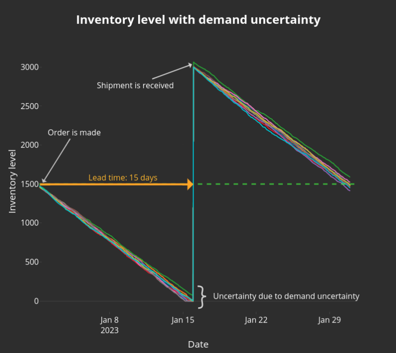

Figure 2: Inventory level over time in the presence of demand (left) or lead time (right) uncertainties. Each curve shows a possible scenario for the level of inventory. Inventory may or may not be replenished before it reaches 0.

Figure 3: Inventory level over time in the presence of both demand and lead time uncertainties. Each curve shows a possible scenario for the level of inventory.
In the presence of uncertainty, the inventory level may reach zero before your shipment arrives, and you will not be able to serve all the demand. Safety stocks are used to mitigate these two sources of uncertainty. Instead you will reorder when you reach a point:
![]()
The more safety stock you have, the higher service level you can expect: the curves of inventory level in Figure 3 will be higher since you reorder when there is more inventory remaining, so it is less likely that your inventory level reaches zero. But how do you choose the quantity of safety stock?
A widely used formula to set safety stocks when we want to reach a particular service level is the following:

In this formula we assume that all quantities are expressed with the same time unit, for example one day:
Now that you know the formula, you might think you just have to perform the computation and that will allow you to set your safety stock level. Before doing that, you must be aware that this formula is valid only when a few assumptions are satisfied:
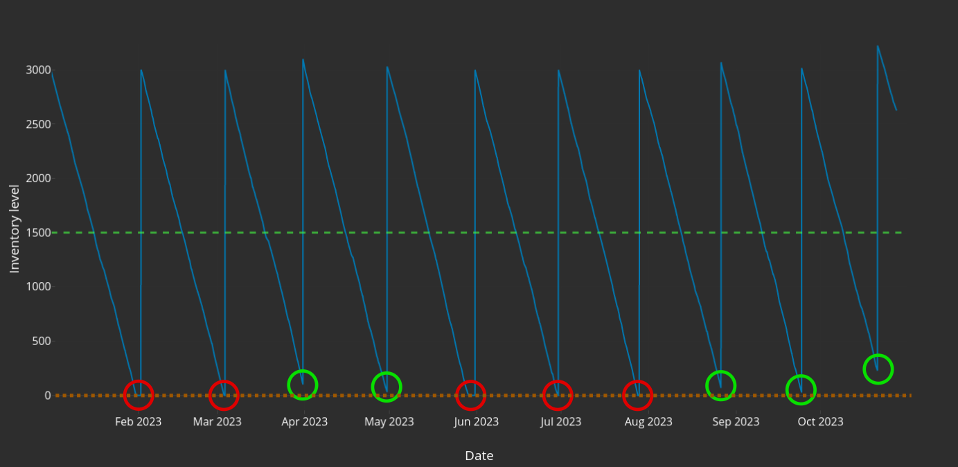 Figure 4: For each replenishment cycle, we observe whether the inventory level reaches 0 (red) or not (green). Out of the 10 replenishment cycles, there are 5 cycles where the inventory level reaches 0, so that not all the demand is fulfilled. The cycle service level in this example is therefore 5/10=50%. The fill rate service level (the fraction of the demand that can be supplied from on-hand inventory) in this example is 98%: while stockouts happen every two cycles on average, they only last for a few days, and only impact a small fraction of the demand.
The safety stock formula has the merit of highlighting the main factors that influence safety stock levels, but it makes strong assumptions that are probably not valid in your supply chain. If you are applying this formula, you should pay particular attention to the last hypothesis and make sure you understand that you are setting safety stocks to reach a particular cycle service level, and not fill rate service level, since the two can be quite different from one another.
Let us use the formula nevertheless. We will assume that your supply chain has the following parameters:
Applying the formula, we get a recommendation for the safety stock of 53.2 refrigerators, which you will round to 53 refrigerators.
Your order point is now 1500+53=1553 refrigerators.
You now expect to reach a cycle service level of 80%. But can you trust the formula? And what is going to be the corresponding fill rate service level? In the next section we are going to simulate your supply chain to understand when you can use the formula, and how much of an impact the different assumptions above really have on your service level.
A simulator is a computer program that mimics the behavior of a real system. In this section we will use a supply chain simulator, which consists in a virtual representation of the supply chain on a computer. The simulator allows to simulate how the supply chain behaves in different circumstances and to test the impact of different safety stocks.
As a starting point we will build a simulator that follows the same hypotheses as the safety stock formula, and use the parameters of the supply chain described above. Later we will remove some of these hypotheses in order to make the simulator closer to reality, and to observe what is the impact on the service level.
The simulator works as follows:
Figure 5: Visualization of the simulation process during the first simulated year.

Figure 6: Final state of the simulation after 10 years. The fill rate service level is 99.8%, while the cycle service level is 80.3%.
After a simulation of 10 years, we measure a simulated cycle service level of 80.3%, and a fill rate service level of 99.8%. The simulated cycle service level is quite close to the target value of 80%, which is expected since we are satisfying the safety stock formula hypotheses in our simulator. Note however that the fill rate service level is dramatically higher. If you were targeting a fill rate of 80%, you shouldn’t apply the formula as you will get a lot of excess inventory (and associated costs).
If we run a new simulation for 10 years we will get slightly different numbers, because of the randomness in the simulation. In order to trust the results completely we can perform an uncertainty analysis. The uncertainty analysis works by running many different simulations and quantifying the uncertainty we have in our predicted service level. The results tell us that the cycle service level for a 10 year period will lie between 75% and 84% with a 95% probability, while the fill rate service level will be between 99.7% and 99.8% with a 95% probability, so our conclusion above remains valid.
Now that we have a simulator we can run different scenarios in which we change the behavior of the supply chain, and observe the impact on the predicted service level.
So far we were working with a continuous review of inventory: at the exact minute where the inventory level goes below the reorder point, the retailer would send an order to his supplier. In this scenario we will assume that the inventory is reviewed only once a day, for example at noon, and we will keep all parameters, including safety stock, the same as in the simulation above. A new simulation is then run.
Figure 7: Final year of the simulation when the inventory is reviewed just once a day.
The total fill rate service level is 99.6%, while the cycle service level is down to 53.8%.
While the fill rate service level hasn’t changed much, going from 99.8% to 99.6%, the cycle service level has completely dropped, from 80% to 53.8%. The cycle service level is very sensitive to such small changes, since a few minutes difference in the arrival of the shipment can be the difference between having a stockout or not during a replenishment cycle. The fill rate service level is less sensitive: even if there is a stockout for a few minutes, only a limited amount of demand will not be served during this time.
If the inventory is reviewed only once a week, the cycle service level drops to 2%, while the fill rate service level drops to 89%.
Let us go back to the initial scenario of continuous review of the inventory. We assumed that the demands on each day were independent of each other. In reality, the demand is correlated with external factors, such as exchange rates, promotions or holidays which persist for longer durations, leading to correlations in time for the demand. This means that the demand on a given day is more likely to be closer to the demand of the previous day, than the demand from several years earlier.
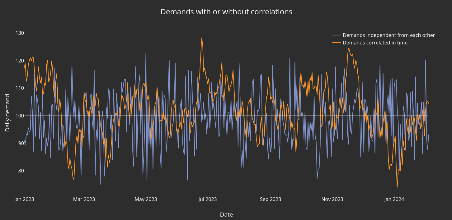
Figure 8: Difference between demands that are independent from each other, and demands that are correlated in time.
In the two cases the daily demand follows a normal distribution with a mean of 100 and a standard deviation of 10.
We now change our simulator so that it generates demands that are correlated in time, while keeping the assumption that the daily demands follow a normal distribution with a mean of 100 and a standard deviation of 10.
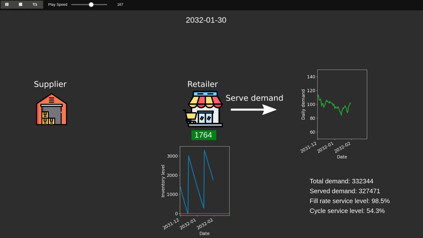
Figure 9: Final year of the simulation when the demands are correlated in time.
The total fill rate service level is 98.6%, while the cycle service level is down to 52.6%.
Once again, changing one of the assumptions of the formula has a dramatic impact on the cycle service level, which drops from 80.3% to 52.6%.
Imagine now that we combine the daily review period with the demands that are not independent of each other. In addition, we realize that the lead times don’t follow a normal distribution, but instead we collect data and observe the distribution depicted on Figure 10, where a few shipments arrive in advance, a lot of shipments arrive with slight delays, and some shipments arrive with longer delays. We know that we cannot trust the formula, since several hypotheses are not valid. But we can still use our simulator, and we can update it so that the lead times follow the distribution observed in the data.

Figure 10: Histogram of measured lead times. The distribution is not normal, so the safety stock formula is not valid, but the simulator can be used with lead times generated from this data.
Our baseline safety stock is 53. By running a simulation we can compute the predicted service level. By now you have realized that the cycle service level is not the metric you are interested in, but you might still wonder how to choose the right amount of safety stock to reach a fill rate service level of 90%.
The first method to find the right safety stock is to run what-if simulations: you start with a safety stock of 53, run a simulation and observe the predicted service level. If it is too low, you will run a new what-if simulation where you increase the safety stock, and if it is too high you will run a new what-if simulation where you decrease the safety stock. After a few simulations you settle on a safety stock of 350, which leads to a fill rate service level of approximately 90%.
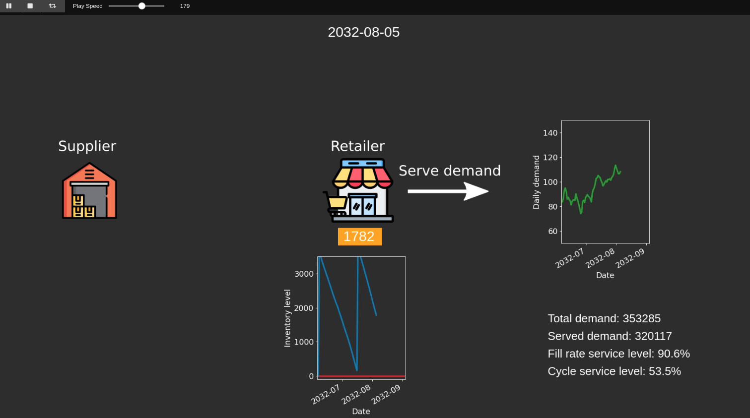
Figure 11: Simulation of a supply chain taking into account realistic lead times.
By removing several assumptions made by the safety stock formula the simulator allows us to represent a more realistic supply chain and the possibilities are endless: you can change the inventory management policy you are using, you can represent not only one supplier but a complex supply chain with multiple suppliers and warehouses, and the cases where no safety stock formula exist can still be simulated.

Figure 12: Simulation of a larger supply chain.
In the previous section we described how we can use a simulator to set the value of our safety stocks. The process requires us to run several simulations until we are satisfied with the predicted service level. Another approach is to automate this process by performing an optimization.
In a simulation the user provides the value of parameters, such as the safety stock, and the simulation returns the predicted value of performance indicators. In the optimization, the user provides instead the target he wants to achieve for his performance indicator (bringing the service level as close as possible to 95%, for example), as well as the levers that the optimizer is allowed to change (the safety stock). The optimizer automatically explores the space of possible choices for the levers, running many simulations along the way.
When it is confident it has found the best possible choice, it returns the corresponding value for the safety stock.
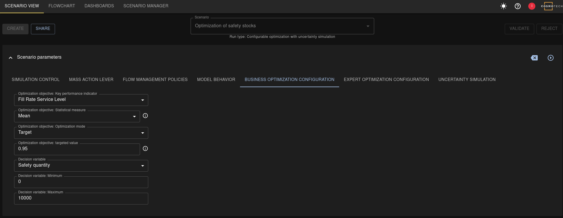
Figure 13: Configuration of a safety stock optimization in the Cosmo Tech supply chain web application
Setting the right amount of safety stocks involves carefully managing the tradeoffs between a higher service level and increased costs. While traditional safety stock formulas have proven effective at highlighting the main factors that influence safety stock levels, they come with their own set of limitations, as they make strong assumptions that are probably not valid in your supply chain.
The complexities inherent in multi-tier supply chains, the ever-present threat of supply chain disruptions, and the increasingly volatile demand further compound this challenge. As such, we need to consider new methods that better align with the current state of our supply chains. By simulating the supply chain under different conditions, managers can gain deep insights into the behavior of their operations. Instead of relying solely on static assumptions, they can test a variety of scenarios and observe the impact on inventory levels, financial indicators and service levels. Using optimization by simulation takes this a step further by harnessing the power of computational algorithms to prescribe the most suitable safety stock level under given circumstances. In a world that is increasingly more complex, unpredictable and competitive, using simulation allows businesses to make informed decisions that improve customer service while reducing costs.